If you haven’t yet heard of Adobe’s Customer Journey Analytics (CJA), it’s a mighty step up from the old world of digital analytics that many of us come from – and it’s completely transforming the way companies analyze and think of their customers’ end to end experience. CJA is powerful in many ways because it sits on top of the Adobe Experience Platform (AEP), which centralizes all the data and applications a company might need to drive the best customer experiences possible.
CJA comes bundled with AEP Query Service, and it’s a convenient way to query the raw data you’ve brought into AEP. I often use it to debug data or inspect it before connecting it to CJA. I also have a confession to make – I don’t know SQL very well, and if I’m honest, I don’t care to learn. R has spoiled me with libraries like dplyr that make interfacing with data a lot easier than SQL ever did (at least in my opinion).
Luckily for people like me, the geniuses behind the R “tidyverse” have come up with dbplyr – a dplyr backend for databases, and it works fantastic with Query Service. Here’s how to get going:
1. Connecting to AEP Query Service
Disclaimer: this setup works for Mac (which I use). If you work on a PC, you can hopefully figure out the essential steps based on what I have below, but you’ll have to try it yourself.
First of all – we’re going to install the package “RPostgreSQL.” If you’ve installed it before, you’ll need to uninstall it. You can do that in R with:
remove.packages("RPostgreSQL")Next, we’ll need to make the following tweaks to your OpenSSL installation. Make sure you have Homebrew installed, and from the Terminal run:
brew uninstall libpq openssl postgresql postgresql@11
brew install libpq openssl postgresql postgresql@11
Then run from the same Terminal:
ln -s /usr/local/Cellar/postgresql@11/11.8_3 /usr/local/Cellar/postgresql/11.8_3
brew switch postgresql 11.8_3
Next, from the RStudio console, you’ll want to run:
install.packages("RPostgreSQL", type="source")
install.packages("dbplyr")
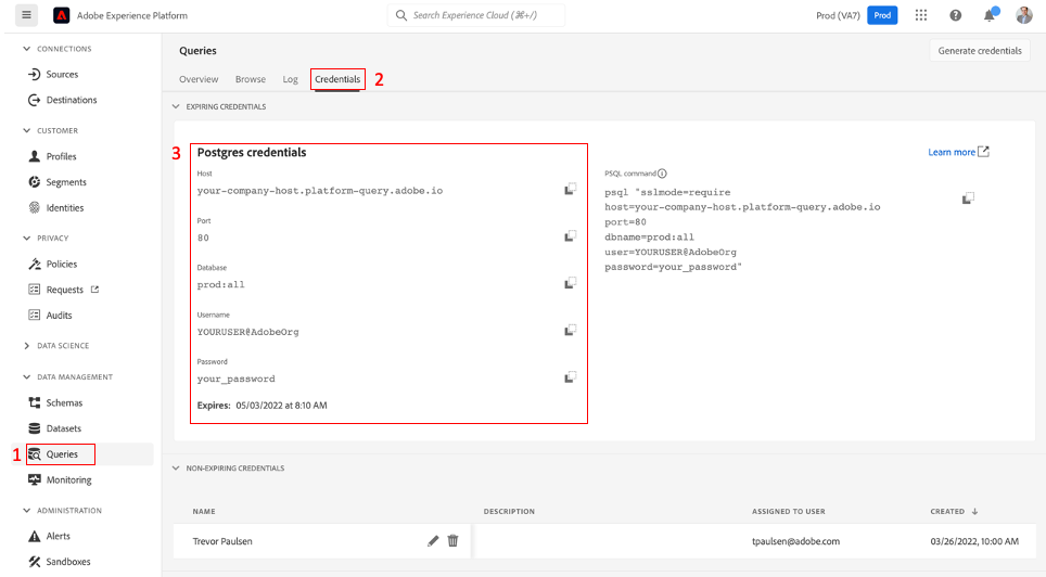
Now that we have that taken care of, we need to grab your Query Service credentials from AEP. You can get those by logging in to AEP and grabbing them from here:

If you want to set up non-expiring credentials, you can find the instructions on setting those up here. Next, we can connect R to Query Service:
require("RPostgreSQL")
library("dbplyr")
library("dplyr")

drv = dbDriver("PostgreSQL")
host = "your-company-host.platform-query.adobe.io"
port = 80
usr = "YOURUSER@AdobeOrg"
pw = "your_password"
con = dbConnect (
  drv = drv,
  dbname = "dbname=prod:all sslmode=require",
  host = host,
  port = port,
  user = usr,
  password = pw
)
on.exit(dbDisconnect(con))
2. Querying data with dbplyr
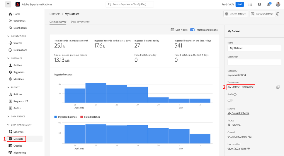
When using dbplyr with Query Service, there are a few helpful tricks that I typically use. First, you need to know the table name of the dataset you want to query. You can find that on the righthand side of your dataset menu:

You can now reference it as a dplyr table and run a simple query to get the number of rows in your dataset:
my_data = tbl(con, "my_dataset_tablename")

my_data %>%
  summarize(
    rows = n()
  )
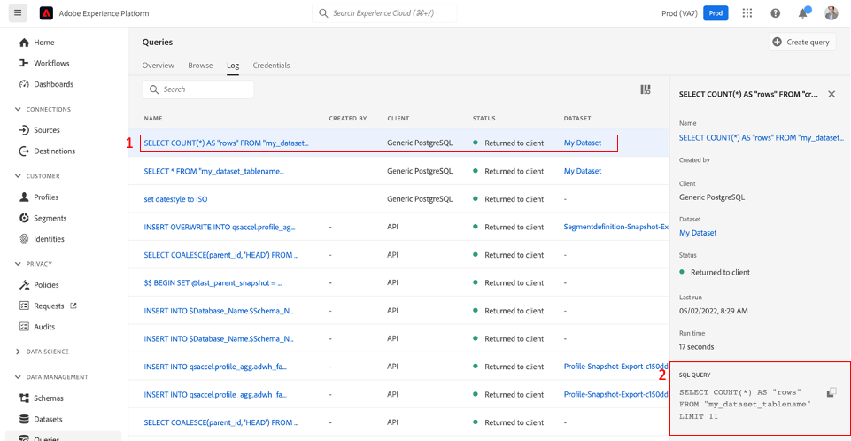
When you run a dplyr statement, you can head over to the Query Log section of AEP, and you’ll notice that dbplyr has converted our dplyr statement into a SQL query and conveniently submitted it to Query Service for us:

Now, we’re ready to have some fun!
One of the most challenging aspects of using a SQL querying tool with modern event-based data is that the schemas are typically complex with lots of field nesting, which is not conducive to SQL. Query Service allows you to use a dot notation to find specific fields (e.g. web.webPageDetails.name to get the page name field) – however, that dot notation is not very friendly to R, which doesn’t support dots or leading underscores in variable names. To get around this, you can use the sql() function coupled with mutate() or transmute() to define the fields you want to create and copy them into more friendly locations:
user_id_sql = sql("endUserIDs._experience.aaid.id")
page_sql = sql("web.webPageDetails.name")
channel_sql = sql("channel._id")

filtered_channel_data = my_data %>%
  transmute(
    user_id = user_id_sql,
    page = page_sql,
    channel = channel_sql
  ) %>%
  filter(user_id == "some_user_id") %>%
  group_by(channel) %>%
  summarize(
    rows = n()
  ) %>%
  collect()
The collect() function is what dbplyr uses to know that you’re ready to execute the query and bring the results back into an R data frame.
Another critical thing to understand is that Query Service does not apply date range filters to your query by default. The query above will query 100% of all data in that dataset. Querying without a date range filter may be too much data for a single query, and the query may take a long time or it may not return at all. To solve this in dbplyr, make sure you add some filtering on the timestamp field:
time_filtered_data = my_data %>%
  filter(timestamp >= to_timestamp("2022-04-01") & timestamp <= to_timestamp("2022-04-30")
3. Chaining queries in dbplyr
One of the most potent aspects of dbplyr is that you can define a set of complex queries without actually executing them, which allows you to chain multiple queries together, but only execute the query once – bypassing the need to create temporary tables. For example, I may want to filter my events down to “all events generated by a person who at any point saw page ABC.”
To accomplish this, we first have to identify all of the user_ids that saw page “ABC,” then join it to the original event table, then filter once again. To do this, we’ll chain a couple of dbplyr query tables:
### Define the list of users I'm interested in
### without running the query yet

user_table = my_data %>%
  transmute(
    user_id = user_id_sql,
    page = page_sql
  ) %>%
  filter(page == "ABC") %>%
  group_by(user_id) %>%
  summarize(
    saw_abc = TRUE
  ) %>%
  ungroup()

### Join the list of users with the event table
### for filtering down the events

filtered_events = my_data %>%
  mutate(
    user_id = user_id_sql
  ) %>%
  left_join(user_table, by="user_id") %>%
  filter(saw_abc) %>%
  collect()
In dbplyr, that’s not too many lines of code – but in SQL, you can see what dbplyr is doing for you under the hood:
SELECT *
FROM   (SELECT "application",
               "channel",
               "timestamp",
               "_id",
               "productlistitems",
               "commerce",
               "receivedtimestamp",
               "enduserids",
               "datasource",
               "web",
               "placecontext",
               "identitymap",
               "marketing",
               "useractivityregion",
               "environment",
               "_experience",
               "media",
               "device",
               "search",
               "advertising",
               "LHS"."user_id" AS "user_id",
               "saw_abc"
        FROM   (SELECT "application",
                       "channel",
                       "timestamp",
                       "_id",
                       "productlistitems",
                       "commerce",
                       "receivedtimestamp",
                       "enduserids",
                       "datasource",
                       "web",
                       "placecontext",
                       "identitymap",
                       "marketing",
                       "useractivityregion",
                       "environment",
                       "_experience",
                       "media",
                       "device",
                       "search",
                       "advertising",
                       enduserids._experience.aaid.id AS "user_id"
                FROM   "my_dataset_tablename") "LHS"
               LEFT JOIN (SELECT "user_id",
                                 true AS "saw_abc"
                          FROM   (SELECT enduserids._experience.aaid.id AS
                                         "user_id",
                                         web.webpagedetails.name        AS
                                         "page"
                                  FROM   "my_dataset_tablename") "q01"
                          WHERE  ( "page" = 'ABC' )
                          GROUP  BY "user_id") "RHS"
                      ON ( "LHS"."user_id" = "RHS"."user_id" )) "q02"
WHERE  ( "saw_abc" )
Barf! The SQL above is why dbplyr is so great – it removes the cognitive overhead that comes with all these nested subselects that are hard to read, hard to write, and easy to mess up.
While that example is elegant, the example I’ve shown here is not typically helpful or feasible. Query Service can only export up to 50 thousand rows at a time, and in my case, I have a lot more than 50 thousand events that I need to analyze. In the next section, I’ll show you how you can output data into another AEP dataset rather than having to collect the data directly in R.
4. Inserting data into an AEP dataset using INSERT INTO
Often I want to create a modified version of a dataset by copying all or some of the events of one dataset into another that I can bring into CJA. For example, I may want to remove some malformed user IDs generated by bots or implementation problems, or I may want to capture events from users that visited some part of my digital property but not other parts. The resulting tables generated by these datasets can be much larger than 50 thousand rows and need to be put into an AEP dataset directly.
To do that, we’re going to use two tricks: 1) the ability to nest a field created in dbplyr into the right schema location using the struct() function and 2) using Query Service’s INSERT INTO ability.
To put data into an AEP dataset, you have to conform strictly to that dataset’s schema, which can be complex and contain nested fields. Unfortunately, SQL is not good at nesting things automatically. For example, I have a field that I’ve created called user_id that I may want to put into the enduserids._experience.aaid.id schema location in my destination dataset. Unfortunately, I can’t just set a field called “enduserids._experience.aaid.id” using dot notation – Query Service will not understand that the field needs to be nested. To solve this, I need to use the struct() function:
query_to_insert = filtered_events %>%
  select(
    # first set the leaf node to the field I created
    id = user_id
  ) %>%
  mutate(
    # now add it to a series of struct fields
    aaid = struct(id),

    # use backticks for variables that start with an underscore
    `_experience` = struct(aaid),

    enduserids = struct(`_experience`)
  ) %>%
  select(
    # select all the fields I want to keep in the destination schema
    enduserids
  )
Using struct() I can get the data into a schema that my destination dataset can understand. Now to finally complete the INSERT INTO I’m going to use a couple of functions to convert my query table (defined by dbplyr) into the SQL that Query Service will understand:
captured_sql = capture.output(show_query(query_to_insert))
sql_needed = paste0(captured_sql[-1], collapse = " ")
dbSendQuery(con, paste0('INSERT INTO destination_table ', sql_needed, ";"))
Since dbplyr doesn’t have a native INSERT INTO function (or other database modifying capabilities), we’ll use the dbSendQuery function to get the job done.
Typically these queries can take quite some time as they have to make a physical write to AEP’s Data Lake, so make sure you’re doing this for date-based chunks of data if needed to avoid timing out.
Summary
Query Service is an excellent tool for inspecting raw data and even has some ability to manipulate and write data into AEP. With R, you can streamline the process using a syntax that is easier to write and read. Hopefully, the tips above will be helpful to you whenever you decide to use AEP Query Service with R. In my next post, I’ll show you how CJA makes pulling data into R even more accessible and powerful using the “cjar” library created by Ben Woodard.
Until then, good luck!
